
You have two policies for a pick-and-place task. Maybe one is a fine-tuned checkpoint and the other is the baseline, or maybe one has an extra camera. You run each of them 50 times. Policy A succeeds 42 times (84%) and policy B succeeds 34 times (68%). Sixteen percentage points is a big gap, so A is better.
Probably. What you actually have is 50 coin flips from each policy, and 50 coin flips wobble. The normal move at this point, when anyone bothers, is to treat the two runs as independent samples and test whether 42/50 and 34/50 could plausibly come from the same underlying success rate. Fisher’s exact test says p = 0.10. Not convincing, so the gap goes into the paper with no error bars and everyone moves on.
That test throws information away, though. If you set the evaluation up carefully, the two policies did not each face 50 random situations. They faced the same 50, with the objects and the arm starting in the same places each time. Once trials are matched like that, “is A better than B?” has a sharper answer, and a psychologist called Quinn McNemar worked it out in 1947 [1].
Four kinds of trial
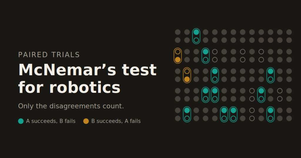
Line the results up by starting layout. For each of the 50 layouts, one of four things happened:
- both policies succeeded
- both policies failed
- A succeeded and B failed
- B succeeded and A failed

This took me longer to accept than it should have. The 33 layouts where both policies succeeded tell you nothing about which policy is better. Neither do the 7 where both failed. Those layouts were easy for everyone or hard for everyone. The comparison lives entirely in the 10 layouts where the policies disagreed, and there A won 9 times and B won once.
Put in the standard 2×2 layout, the counts look like this:
| B succeeds | B fails | |
|---|---|---|
| A succeeds | a = 33 | b = 9 |
| A fails | c = 1 | d = 7 |
The success rates are (a + b)/n for A and (a + c)/n for B. Their difference is (b − c)/n. The a cancels. So does d. The only numbers that matter are the two off-diagonal cells, which statisticians call the discordant pairs.
The test is a coin flip
Now suppose the two policies are equally good. On any layout where they disagree, which one comes out ahead should be a coin toss. So out of b + c = 10 disagreements, the number A wins should look like 10 flips of a fair coin.
Getting 9 or more heads (or 9 or more tails) from 10 fair flips has probability 22/1024, about 0.021. That is the exact McNemar test. It is a binomial test on the disagreements and nothing else.
from scipy.stats import binomtest
from statsmodels.stats.contingency_tables import mcnemar

# rows: A succeeded / A failed    columns: B succeeded / B failed
table = [[33, 9],
         [ 1, 7]]

print(mcnemar(table, exact=True).pvalue)        # 0.0215

# the same thing, spelled out
b, c = table[0][1], table[1][0]
print(binomtest(b, n=b + c, p=0.5).pvalue)      # 0.0215
If you log per-episode outcomes as boolean arrays, one entry per starting layout and in the same order for both policies, building the table is four lines:
import numpy as np

def paired_table(a_ok, b_ok):
    a_ok, b_ok = np.asarray(a_ok, bool), np.asarray(b_ok, bool)
    return [[np.sum(a_ok & b_ok),  np.sum(a_ok & ~b_ok)],
            [np.sum(~a_ok & b_ok), np.sum(~a_ok & ~b_ok)]]
McNemar’s original paper used a chi-squared approximation, (b − c)² / (b + c), with one degree of freedom. Most textbooks quote a version with Edwards’ continuity correction, (|b − c| − 1)² / (b + c) [3], which here gives 4.9 and p = 0.027. With counts this small I would use the exact version. It is also worth knowing that the exact test is conservative, meaning it rejects less often than its nominal rate. Fagerland, Lydersen and Laake compared the variants and recommend the mid-p version (p = 0.012 here) or the uncorrected chi-squared over the exact conditional test [4]. Whichever you pick, pick it before you look at the numbers.
Machine learning has been here before. Dietterich’s comparison of tests for machine learning classifiers recommended McNemar’s test for comparing two models on a single test set, because it kept false positives under control where the popular alternatives did not [2]. A test set of images and a set of 50 starting layouts are the same thing in the respect that matters: both models see identical inputs.
Same headline, different answer
The reason all of this matters is that the headline numbers, 84% against 68%, are compatible with very different stories.
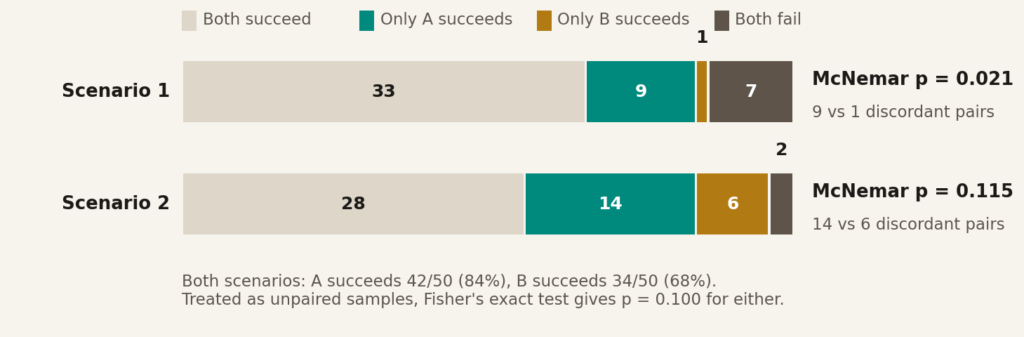
In scenario 1 the policies mostly agree about which layouts are hard. A fixes nine of B’s failures and introduces one of its own. That is a clean, consistent improvement, and McNemar gives p = 0.021, stronger than the p = 0.10 you got by ignoring the pairing.
In scenario 2 the policies fail on largely different layouts. A beats B fourteen times but B beats A six times, and fourteen against six is the sort of split a fair coin produces more often than people expect. McNemar gives p = 0.115. You would get a similar picture from the approximate 95% confidence intervals for the difference in success rate: roughly +4 to +28 points in scenario 1, and roughly −1 to +33 in scenario 2. (Those are simple Wald intervals, which are rough at these sample sizes; better-behaved intervals exist, but the contrast survives.)
Scenario 2 actually comes out slightly worse than the unpaired test, which surprised me the first time. Pairing buys you power only when outcomes on the same layout are correlated, when a layout that is hard for B also tends to be hard for A. Scenario 2 is close to what you would expect if the two policies’ outcomes were unrelated, and in that case matching trials gives you nothing to work with. In practice robot policies trained on similar data usually do share hard cases (the cluttered bin, the object right at the edge of the workspace), which is why pairing tends to help.
Five disagreements are never enough
There is a hard floor hiding in the coin-flip view. Suppose A wins every disagreement. The smallest p-value the exact test can produce with k discordant pairs is 2 × 0.5^k.
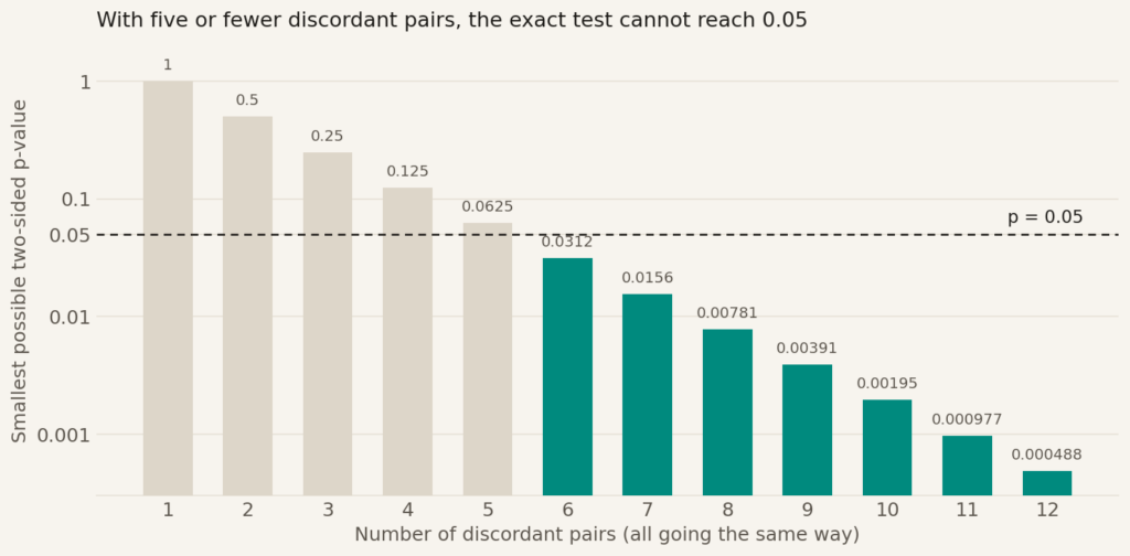
With five disagreements, all going A’s way, the best you can do is p = 0.0625. You need at least six before significance at the 5% level is even possible. Two policies that agree on 48 of 50 layouts and split 2–0 on the rest are, statistically, indistinguishable, and no choice of test will change that.
This is also why the total number of trials is a misleading measure of how much evidence you collected. Two strong policies on an easy task might agree on 95 out of 100 layouts. That leaves five disagreements, and you have learned very little about which one is better, however long the evaluation took. If you are planning trials, what you are really budgeting for is discordant pairs. When you expect the policies to agree a lot, you either need many more trials or harder layouts that actually separate them.
Making the pairing real
All of this assumes the trials really are matched, and it is easy to break that without noticing.
In simulation, pair on the environment. Use the same list of initial states, in the same order, for both policies. Benchmarks such as LIBERO ship a fixed set of initial states for each task [7], so evaluations on it are already paired, whether or not the paper treats them that way. Policy sampling noise (from a diffusion or flow-matching head, say) is part of what you are measuring, so do not try to “match” it between two different policies.
On hardware it takes more effort. Photograph the scene or tape a template to the table, reset, run A, reset to the same layout, run B. Flip a coin for which policy goes first on each layout. If you can, keep whoever judges success from knowing which policy they are watching. Deciding whether a half-completed grasp counts is more subjective than anyone likes to admit.
Running the two back to back also protects you from drift. The light through the lab window in the afternoon is not the light in the morning, gripper pads wear, and someone always nudges a camera eventually. If you run all of A on Monday and all of B on Tuesday, every one of those differences is folded into your comparison and nothing in the data will tell you. Run each pair within a few minutes and slow drift hits both policies about equally, so the pairing cancels it.
Finally, decide how many trials you will run before you start. Running layouts until p drops below 0.05 and then stopping inflates the false positive rate badly. If you want to stop early legitimately, there are sequential methods built specifically for robot policy comparison [6]. Kress-Gazit and colleagues’ paper on evaluation practice is also a good, readable argument for treating evaluation as experiment design rather than bookkeeping [5].
Where McNemar stops
The test answers one narrow question. Across these matched trials, does one policy succeed more often than the other? Real evaluations usually want a bit more than that.
If you are comparing more than two policies on the same layouts, Cochran’s Q test is the generalisation [8], and with two policies it reduces to McNemar’s. Running every pairwise McNemar test is also fine as long as you correct for the number of comparisons. Holm’s method is the easy default.
With several tasks, you can pool pairs across the suite, since each pair is still a pair. The test then tells you whether A is better on average, which can hide a policy that is much better on three tasks and worse on two. If the per-task picture matters, test each task and correct for multiple comparisons. At 50 trials per task, expect those tests to be weak.
McNemar only sees success or failure. If you score partial progress, such as subgoals reached, use a paired test built for graded scores, like the Wilcoxon signed-rank test or the plain sign test. McNemar is really the sign test with binary outcomes, so this is the same idea stretched a little.
And a tiny p-value is not the same as a useful improvement. Run 2,000 simulated episodes and a one-point gain nobody would bother deploying can come out as highly significant. I would always report the difference with an interval and treat the p-value as supporting evidence.
These days, whenever I see two success rates side by side in a paper, I go looking for the 2×2 table. It is rarely there, which is a shame, because the 9 and the 1 would tell me more than the 42 and the 34.
References
[1] Q. McNemar, “Note on the sampling error of the difference between correlated proportions or percentages,” Psychometrika, vol. 12, no. 2, pp. 153–157, 1947, doi: 10.1007/BF02295996.
[2] T. G. Dietterich, “Approximate statistical tests for comparing supervised classification learning algorithms,” Neural Computation, vol. 10, no. 7, pp. 1895–1923, 1998, doi: 10.1162/089976698300017197.
[3] A. L. Edwards, “Note on the ‘correction for continuity’ in testing the significance of the difference between correlated proportions,” Psychometrika, vol. 13, no. 3, pp. 185–187, 1948.
[4] M. W. Fagerland, S. Lydersen, and P. Laake, “The McNemar test for binary matched-pairs data: mid-p and asymptotic are better than exact conditional,” BMC Medical Research Methodology, vol. 13, art. no. 91, 2013, doi: 10.1186/1471-2288-13-91.
[5] H. Kress-Gazit et al., “Robot learning as an empirical science: Best practices for policy evaluation,” arXiv:2409.09491, 2024.
[6] D. Snyder et al., “Is your imitation learning policy better than mine? Policy comparison with near-optimal stopping,” arXiv:2503.10966, 2025.
[7] B. Liu et al., “LIBERO: Benchmarking knowledge transfer for lifelong robot learning,” in Advances in Neural Information Processing Systems, vol. 36, 2023.
[8] W. G. Cochran, “The comparison of percentages in matched samples,” Biometrika, vol. 37, no. 3/4, pp. 256–266, 1950.