
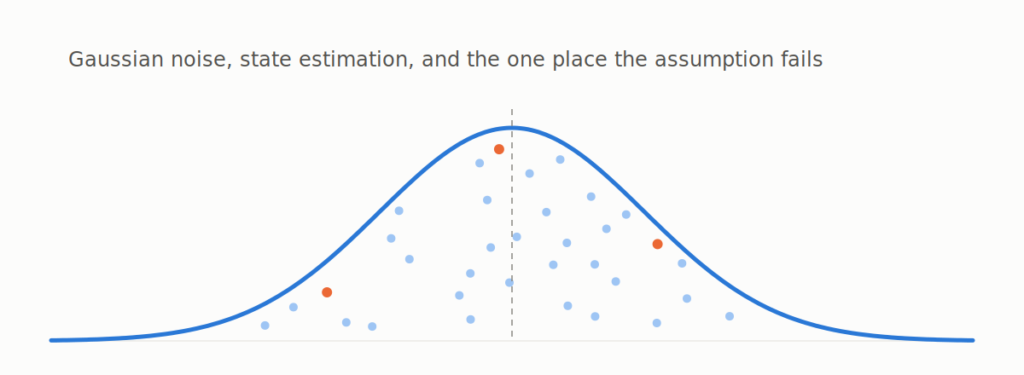
Point a laser rangefinder at a wall exactly one metre away and take a thousand readings. You will not get a thousand identical numbers. You will get a cloud sitting around one metre: 0.997, 1.004, 1.001, 0.995, and so on. Plot those in a histogram and out comes a shape everybody recognises, the symmetric hump that turns up in exam results and human heights and pretty much every measurement anyone has ever taken.
That hump is a Gaussian, also called a normal distribution. It is described by two numbers: where the centre sits (the mean) and how wide it spreads (the standard deviation, sigma). Roughly 68% of readings land within one sigma of the mean and about 95% within two.
Simulating it takes one line:
import numpy as np

true_distance = 1.00   # metres
sigma = 0.004          # 4 mm of sensor noise

readings = np.random.normal(true_distance, sigma, size=1000)
print(readings[:5])
print(readings.mean(), readings.std())
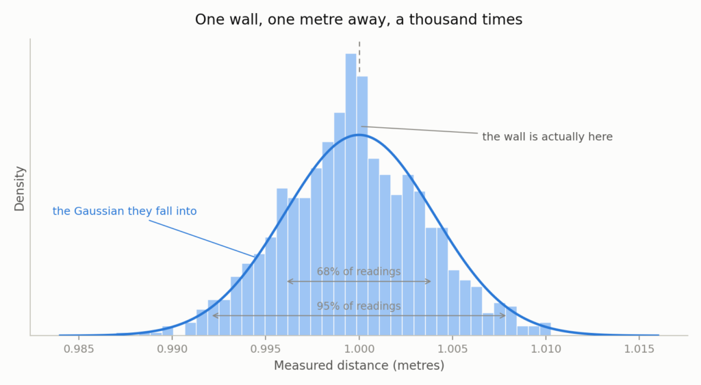
Any single reading might come back as 1.006. The mean of a thousand of them will sit very close to 1.0000. That is the first genuinely useful property of Gaussian noise: it averages away. The error in your estimate shrinks with sigma over the square root of n, so four times the readings buys you half the error. Diminishing returns, and it only works if the noise is truly random rather than a bias. If your sensor reads 3 mm long because it warmed up, no amount of averaging will save you. It will just give you a very precise wrong answer.
Why Gaussians rather than some other shape
There are two reasons. One is respectable and one is pragmatic, and I think it is worth being honest about which does more of the work.
The respectable reason is the central limit theorem. The error in that rangefinder is not one thing. It is thermal noise in the photodiode, timing jitter in the electronics, a bit of vibration through the mount, some dust in the air, the wall not being perfectly flat. Add up many small independent errors and the total tends towards a Gaussian no matter what the individual pieces looked like. So bell curves genuinely do fall out of the physics quite often.
The pragmatic reason is that Gaussians are extraordinarily well behaved. Add two Gaussian variables and you get a Gaussian. Push one through a linear function and it stays Gaussian. Multiply two Gaussian densities and the result is proportional to yet another Gaussian. Almost nothing else in probability is that tidy. It means a robot can carry its entire belief about where it is in two numbers and update them with a handful of arithmetic, instead of running a simulation.
In practice the second reason wins far more arguments than papers tend to admit. We assume Gaussian because the maths closes cleanly, not because somebody plotted the histogram and checked.
A robot does not know where it is. It has an opinion.
This is the mental shift that made everything else click for me. A robot does not have a position. It has a belief about its position, and that belief is a distribution. “I am at x = 4.2 metres, give or take 0.3” is a complete statement. “I am at 4.2 metres” is not, because it hides the bit you need in order to decide whether to trust it.
Two things then happen over and over, forever.
The robot moves, and the belief gets worse. Odometry says the wheels turned enough for half a metre, but the carpet had a fold in it and one wheel slipped. So you add motion noise, and the variance grows.
The robot senses, and the belief gets better. A landmark, a GPS fix, a wall at a known distance. Uncertainty shrinks.
A Kalman filter is those two steps in a loop, and in one dimension it is genuinely this small:
def predict(mu, var, motion, motion_var):
    """Robot moved. We are now less sure."""
    return mu + motion, var + motion_var

def update(mu, var, meas, meas_var):
    """Sensor spoke. We are now more sure."""
    k = var / (var + meas_var)          # Kalman gain
    return mu + k * (meas - mu), (1 - k) * var
The interesting line is the gain, k. It sits between 0 and 1 and it decides how much to believe the sensor. If your belief is already sharp and the sensor is noisy, k comes out near zero and the reading barely moves you. If you are hopelessly lost and the sensor is precise, k goes near one and you jump straight to the measurement. Nobody tunes this by hand. It falls out of the two variances.
Run it and watch what happens:
mu, var = 0.0, 1.0

for step in range(10):
    mu, var = predict(mu, var, motion=0.5, motion_var=0.05)
    z = np.random.normal(0.5 * (step + 1), 0.3)   # noisy position fix
    mu, var = update(mu, var, z, meas_var=0.09)
    print(f"step {step}:  x = {mu:.2f}  ±{np.sqrt(var):.2f}")
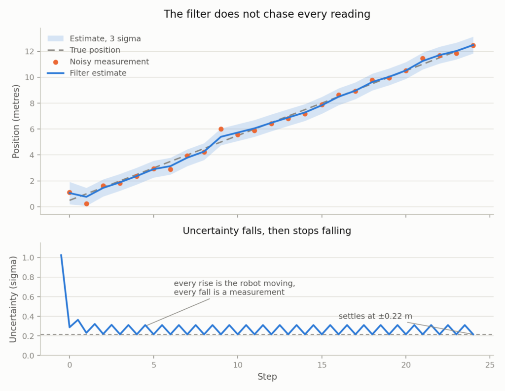
Watch the bottom panel and you can see the loop breathing. Every rise is motion adding doubt, every fall is a measurement taking some back. The uncertainty drops fast at first and then stops dropping. It does not go to zero. It settles at around 22 centimetres, the point where the doubt gained by moving exactly balances the doubt removed by sensing, and that equilibrium is, more or less, how accurate your robot actually is. If you want it better you have to buy a quieter sensor or slip less. There is no third option.
Real systems are messier, obviously. Position, velocity and orientation together, so the two numbers become a mean vector and a covariance matrix, and the off-diagonal terms encode useful things like “I am unsure how fast I am going, so I am also unsure where I will be next”. Nonlinear dynamics need the extended or unscented variants, which linearise or sample their way around the problem. The shape of it stays the same.
Noise you add on purpose
So far noise is something happening to the robot. Half of modern robotics does the opposite and adds it deliberately.
Take simulation. Training a policy in sim is cheap and safe and fast, and the trouble is that sim is far too clean. Depth images are perfect. Friction is exactly the number you typed. Every joint reaches precisely the angle you commanded, on time. A policy trained in that world quietly learns to depend on precision it will never have once it is on real hardware, and then it falls over in the lab.
The fix is to wreck the simulation on purpose. Jitter the camera pose, add Gaussian noise to joint readings, randomise link masses and friction coefficients each episode:
obs_noisy = obs + np.random.normal(0, 0.02, size=obs.shape)
Two lines, and the policy can no longer memorise one exact world. It has to find a strategy that survives across the whole spread. This is domain randomisation, it is about as blunt as an instrument gets, and it works considerably better than it has any right to.
Reinforcement learning uses Gaussians in a second way. A continuous-control policy usually outputs a mean action and a standard deviation, then samples from that distribution rather than acting on the mean. The sigma is the exploration. Start it wide so the robot flails about and discovers things, shrink it as the policy gets confident. Set it to zero at the start and the robot does the same slightly wrong thing forever.
Then there are diffusion policies, which are the ones I keep turning over in my head. You take an expert demonstration and destroy it, adding Gaussian noise step by step until the action sequence is pure static. Then you train a network to run that destruction backwards. At deployment you start from noise and denoise your way into a trajectory. Noise stops being the thing you fight and becomes the raw material you shape.
It also handles a problem that quietly ruins simpler methods. If there are two sensible ways round an obstacle, left and right, a model trained to predict the average demonstration will happily output the average of left and right, which is straight into the obstacle. A diffusion model represents both routes as separate modes and samples one of them.
Where the assumption bites back
Which brings me to the failure cases, because a bell curve is a strong claim about the world and sometimes it is simply false.
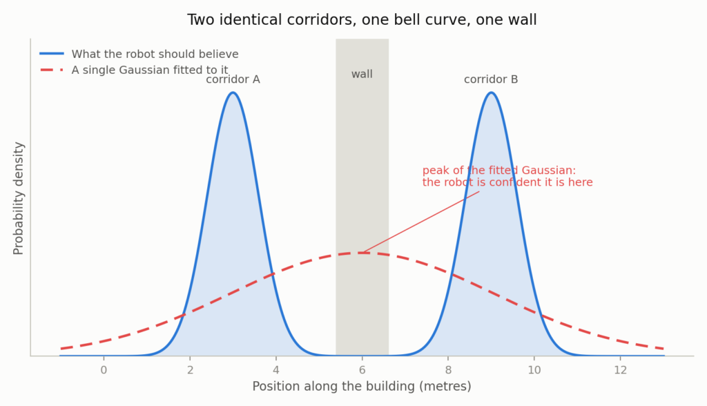
The worst one is multimodality. Put a robot in a building with two identical corridors and its honest belief is “I am in corridor A or corridor B”, two separate humps. Force a single Gaussian onto that and you get a mean sitting neatly between them, which is inside a wall. The robot is now confident about a location it cannot possibly occupy, and confidence is what makes it dangerous rather than merely wrong.
Then there are outliers. A lidar beam hits a window, or somebody walks in front of the sensor. Under a Gaussian, a reading twenty sigma from the mean is so improbable it may as well be forbidden, so when one turns up the filter interprets it as enormously informative and lurches. Real systems patch this with gating, robust loss functions or heavier-tailed distributions like Student’s t, all of which amount to admitting the tails are fatter than the model claims.
And Gaussians run to infinity in both directions, which is fine for position and silly for anything bounded. Battery charge cannot be negative. A joint cannot exceed its mechanical limit. Usually this causes no trouble at all, right up until it produces a state estimate of minus three percent charge and something downstream divides by it.
None of this makes the Gaussian assumption wrong. It makes it a modelling choice with a price attached, and knowing the price is most of the skill. My rough test: if the thing I am uncertain about could reasonably have two answers rather than one fuzzy answer, a bell curve is going to lie to me. It will do it with a small variance and a completely straight face.